In this article, I’ll be presenting the results and part of the development process of our current goals probability model.
Defining the problem
First of all, I will explain our approach to the problem of predicting goals in a match. When building a prediction model, one must first decide if it will make predictions during the game or only before it happens. Of course, the model that predicts in-play matches will also be capable of making predictions before it starts (t=0), and for this reason, we chose to develop this kind of model.
Technically speaking, our model would have numerous independent variables, called features in AI models, as inputs and in addition, the relative number of goals that we would like to get the probability. An example is shown below.

Ch=corners home, Ca=corners away
Preparing the data
To solve the problem we chose to use machine learning models because the relationships between the independent variables and the target variable are unknown and often very complex. Additionally, we are not interested in deriving conclusions from the data model itself (i.e: how is the relationship between independent and target variables), but only interested in getting the output.
As discussed in the great article The Wisdom of the Crowd, the best way to estimate the probabilities of a given event in football would be to ask numerous bettors to estimate the probabilities themselves. Luckily, this is translated to the odds of a given market for a bookmaker or a betting exchange. As you may know, the odd is related to the implied bookmaker probability by the following equation:
odd = 1/probbm
The implied bookmaker probability is related to the fair probability by the following equation:
∑probfair + M = ∑probbm
where M is the bookmaker’s margin.
Solving this equation we can get to an approximation of the fair probability calculated by the bookmaker. This result is the target of our model and was used to train it.
Training the model
The model was trained using many stats from the match, both live stats and pre-live stats and had the fair probability of the game ending with the specified amount of total goals as an output. The dataset was divided into two sets, the training set and the test set, as is usual for machine learning models. The key point here was that this division made sure that the matches in the test set were not found in the training set, as this would be considered data leakage.
Additionally, the model was tuned to use the best hyperparameters using grid search, always sorting the results by the loss function, in this case, the mean squared error function. Below are the results of the best model configuration on the test set.
| Metric | Value |
| Mean Absolute Error | 0.024 |
| Mean Squared Error | 0.00089 |
| Mean Error | -0.0039 |
| Standard deviation of error | 0.03 |
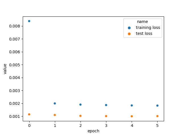
We can see above that the training loss decreases a lot at the start of training and the test loss is very small already at the start. At first glance, this plot does not seemed right. (1) This is seemed to be an example of a model that has the learning rate set too high: the model adjusts a lot to the data on the first epoch and after that the learning rate is so high that the model cannot learn anything anymore. (2) It’s also, strange at first, that the test loss is much lower than the training loss on the first epoch.
Regarding (1), some factors should be considered first: 1. the training set is huge and 2. the test loss is calculated after the first epoch of training. If the model has learned everything it can from the data on the first epoch, the validation loss is expected to be a lot lower than the training loss (remember that the loss is calculated at the end of every batch processing, even when the model is very “dumb”).
This begs the question: Why use this configuration then? Why not use a lower learning rate? The answer is: because after testing exhaustively the model with various configurations, the one that better performed had the chosen configuration, although the majority didn’t have much differing performance.
Now regarding (2), the fact that the testing loss is lower than the training loss on later epochs is due to the fact that regularization was used when training the model. As you may know, regularization is used when training but not when predicting. This is well explained by this thread.

The distribution of the errors can clearly be seen as normal, as one would expect, with the mean and standard deviation described above. With this information, we can conclude that approximately 95% of the errors will fall between -5.2pp and 4.4pp of difference from the true probability. This is a very interesting result, especially considering that bookmakers and betting exchanges have an average of 2.5pp of difference between their implied probability and even can present differences much higher.