Why Transformers Changed Everything: Input Embeddings

To understand how a Transformer works, let’s dissect the diagram below that shows all the steps in the process.
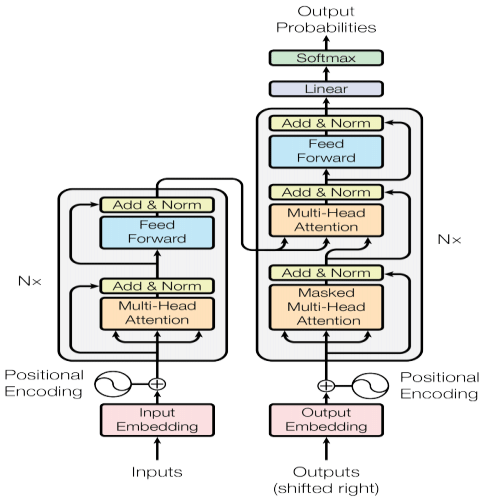
Mechanism of the Transformer. (https://www.researchgate.net/figure/1-Mechanism-of-the-Transformer_fig2_340659282)

Input embeddings

When we talk about the use of neural networks and more broadly machine learning techniques, we work exclusively with numbers. What I mean by this is that any type of unstructured data, or even structured data, but in the form of text, for example, has to first be transformed into numbers so that it can be “learned” by machine learning models.

Hence the question arises: how to transform text into numbers?

Bag of words

There are some ways to do this, and new alternatives have been discovered to try to solve this problem. One of the first solutions found was to give a “position” to each word and count the number of appearances of each word in the input text, a technique called bag of words. The image below demonstrates how this is done: each word has a position in the table below (each vocabulary word is a column) and the value of each cell is the count of how many times each word appeared in the input text, represented by the lines.

BOW on Surfin’ Bird (https://openclassrooms.com/en/courses/6532301-introduction-to-natural-language-processing/8081284-apply-a-simple-bag-of-words-approach)

Then another question may arise: why not associate an identifier with each word and have a matrix in which the values are the index (or identifier of each word) and the columns are the position of each word in the text, for example? Due to the nature of neural networks (and most machine learning techniques) the features, in the example above the columns, are always quantitative variables. In other words, if I say that the word “I” has the identifier 1 and the word “you” has the identifier 2, this does not mean that “you” is greater than “I”, because despite 1 < 2, these numbers are just identifiers. However, a model would “understand” that this would be quantitative data, generating enormous confusion and making it impossible to arrive at a satisfactory result for real applications.

Words as vectors

To solve the problems mentioned above, some alternatives were proposed with one main idea in mind: words that appear together have similar meanings and similar contexts. The idea here is that words can be represented according to n arbitrary characteristics. To illustrate this idea, we have the following example: the word “taxes” and the word “interest” are both words widely used in contexts of financial texts, therefore, we could define a quantity that would be the “finance score”, that is, how much a word is used in the context of financial texts, and its domain would be between 0 and 1, the closer it is to 1, the more this word is used in this context. The two words mentioned would certainly be close to 1, which indicates that if we created n quantities, we could classify all words in the vocabulary and similar words would have similar values for these quantities.

In this line of thought, algorithms such as GloVe: Global Vectors for Word Representation emerge, which represent words in n dimensions in space. These dimensions do not have any meaning that can be easily interpreted by us human beings, such as “finance score”, but for models these meanings exist.

This is the first stage of a Transformer and of great importance! See you in the next step, positional encoding.

Predicting football match goals with an AI model

In this article, I’ll be presenting the results and part of the development process of our current goals probability model.

Defining the problem

First of all, I will explain our approach to the problem of predicting goals in a match. When building a prediction model, one must first decide if it will make predictions during the game or only before it happens. Of course, the model that predicts in-play matches will also be capable of making predictions before it starts (t=0), and for this reason, we chose to develop this kind of model.

Technically speaking, our model would have numerous independent variables, called features in AI models, as inputs and in addition, the relative number of goals that we would like to get the probability. An example is shown below.

Model Overview: Gh = goals home, Ga=goals away,
Ch=corners home, Ca=corners away

Preparing the data

To solve the problem we chose to use machine learning models because the relationships between the independent variables and the target variable are unknown and often very complex. Additionally, we are not interested in deriving conclusions from the data model itself (i.e: how is the relationship between independent and target variables), but only interested in getting the output.

As discussed in the great article The Wisdom of the Crowd, the best way to estimate the probabilities of a given event in football would be to ask numerous bettors to estimate the probabilities themselves. Luckily, this is translated to the odds of a given market for a bookmaker or a betting exchange. As you may know, the odd is related to the implied bookmaker probability by the following equation:

odd = 1/probbm

The implied bookmaker probability is related to the fair probability by the following equation:

probfair + M = probbm

where M is the bookmaker’s margin.

Solving this equation we can get to an approximation of the fair probability calculated by the bookmaker. This result is the target of our model and was used to train it.

Training the model

The model was trained using many stats from the match, both live stats and pre-live stats and had the fair probability of the game ending with the specified amount of total goals as an output. The dataset was divided into two sets, the training set and the test set, as is usual for machine learning models. The key point here was that this division made sure that the matches in the test set were not found in the training set, as this would be considered data leakage.

Additionally, the model was tuned to use the best hyperparameters using grid search, always sorting the results by the loss function, in this case, the mean squared error function. Below are the results of the best model configuration on the test set.

MetricValue
Mean Absolute Error0.024
Mean Squared Error0.00089
Mean Error-0.0039
Standard deviation of error0.03
Metrics on the test set
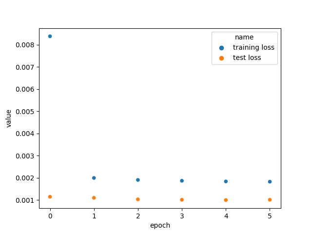
Training and testing set loss

We can see above that the training loss decreases a lot at the start of training and the test loss is very small already at the start. At first glance, this plot does not seemed right. (1) This is seemed to be an example of a model that has the learning rate set too high: the model adjusts a lot to the data on the first epoch and after that the learning rate is so high that the model cannot learn anything anymore. (2) It’s also, strange at first, that the test loss is much lower than the training loss on the first epoch.

Regarding (1), some factors should be considered first: 1. the training set is huge and 2. the test loss is calculated after the first epoch of training. If the model has learned everything it can from the data on the first epoch, the validation loss is expected to be a lot lower than the training loss (remember that the loss is calculated at the end of every batch processing, even when the model is very “dumb”).

This begs the question: Why use this configuration then? Why not use a lower learning rate? The answer is: because after testing exhaustively the model with various configurations, the one that better performed had the chosen configuration, although the majority didn’t have much differing performance.

Now regarding (2), the fact that the testing loss is lower than the training loss on later epochs is due to the fact that regularization was used when training the model. As you may know, regularization is used when training but not when predicting. This is well explained by this thread.

Histogram of errors on the test set

The distribution of the errors can clearly be seen as normal, as one would expect, with the mean and standard deviation described above. With this information, we can conclude that approximately 95% of the errors will fall between -5.2pp and 4.4pp of difference from the true probability. This is a very interesting result, especially considering that bookmakers and betting exchanges have an average of 2.5pp of difference between their implied probability and even can present differences much higher.

Why transformers changed everything: LSTMs

After seeing the problems of the simple RNNs seen before researchers proposed a new approach to memory-related models. The new approach was named the LSTM model.

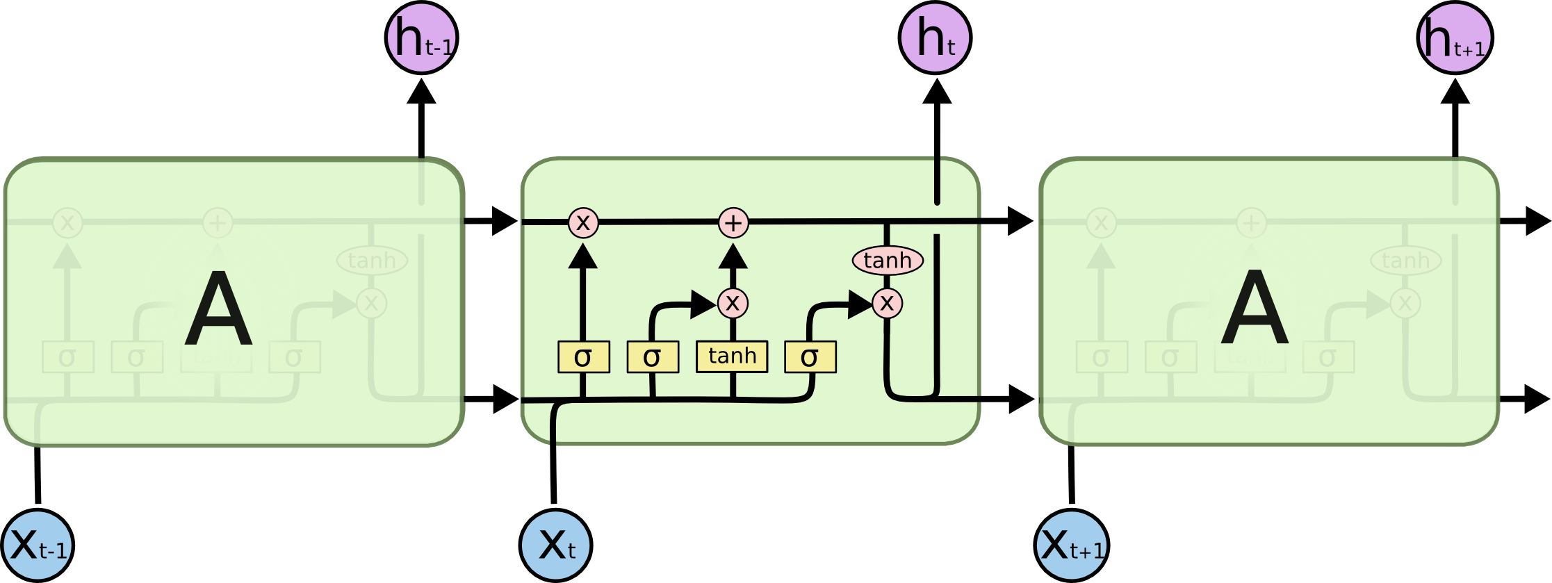
Long Short Term Memory architecture (LSTM)

Although the LSTM models are a variant of the Recurrent Neural Networks, they have very important changes. The whole idea is to separate the cell state from the current input values.

Source: https://colah.github.io/posts/2015-08-Understanding-LSTMs/

The top horizontal line is called the state of the cell, this is considered the long-term “memory” of the cell. Another special component of the architecture are the gates. Whenever you see a multiplication sign it means that it is a gate.

Source: https://colah.github.io/posts/2015-08-Understanding-LSTMs/

Gates

In this case, they are preceded with a sigmoid activation function and the explanation for that is that the sigmoid function output goes from 0 to 1, therefore, the multiplication operation works as a gate for letting some information pass to the next stage or be forgotten. This way, the cell state can be changed and only the important things at the moment are remembered by the model.

The output

The output of the model is the value h, which can be viewed as a filtered version of the state of the cell. It is filtered at the last gate on the right, which has as input the cell state passed through a tanh function.

Other variants

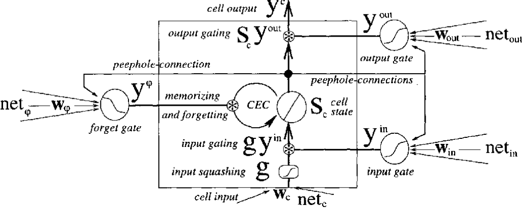
Peephole connections

Introduced by Gers & Schmidhuber (2000), the peephole approach provides the gates with the cell state itself as an input.

Source: https://d3i71xaburhd42.cloudfront.net/545a4e23bf00ddbc1d3325324b4c61f57cf45081/2-Figure1-1.png
Gated Recurrent unit (GRU)

Introduced by Cho, et al. (2014), it merges the input and the forget gates into one gate, called the “update gate”. This achieves a simpler architecture, being easier to train and computationally cheaper. This variant has gained a lot of popularity over the years.

Source: https://colah.github.io/posts/2015-08-Understanding-LSTMs/

Conclusion

The introduction of the LSTM architecture brought far more possibilities to solve problems. The model proposed, and its variants, have been used successfully with various memory-related solutions.

The next big step that will be discussed in the next article is the Attention architecture introduced by Google. An approach that, again, changed everything in the machine learning world and created many more possibilities.

Why transformers changed everything: before

In this series of articles I will discuss why the invention of transformers, published by the Google’s AI team in the paper titled Attention Is All You Need (2017) was so important to machine learning and the deep learning fields.

First of all, to understand the accomplishments of these proposed ideas, one must first understand how things were done before. We all know that context matters, in some cases, it matters a lot. For example, while reading this article, you keep all the text that came before in mind to comprehend the next sentences, otherwise it wouldn’t make any sense to you.

Of course, it doesn’t take long to one arrive to the conclusion that there can be a lot of concerns when dealing with context. Continuing with reading as an example, how long is your context? In other words, how many sentences (or ideas) back do you remember from a text in order to make sense of it? This answer cannot be other than that the context varies in length. So how can we input that into a model?

Using a neural network with words at their respective positions as input would not work as the model would have to have a fixed input size and we established that a context can’t have a fixed length. One of the first ideas was to use RNNs or Recurrent Neural Networks.

Recurrent Neural Networks

These are neural networks that look like this:

The h in the image is simply an activation function and weights. x are the inputs at each state and o is the prediction output for that state. The important thing to notice here is that the weights are equal between all the units of the network. This grants the following advantages to the model:

  1. Information about past states is used by the network to calculate the output (prediction) of the model;
  2. The quantity of past states can vary indefinitely;
  3. The model is very computationally efficient and therefore are easily trained.

Unfortunately, although the advantages of this type of model seem great there are some deal-breaker problems with this approach:

  1. The information from past several states is almost entirely lost and becomes practically unavailable at the last step of the calculation (the last layer);
  2. This model suffers from the Vanishing/Exploding gradient problem.

These limitations restrict the use cases of this method to situations where the number of past states to be considered is relatively very small. However, the proposed architecture can be changed to fix these problems.

Vanishing/Exploding gradient problem

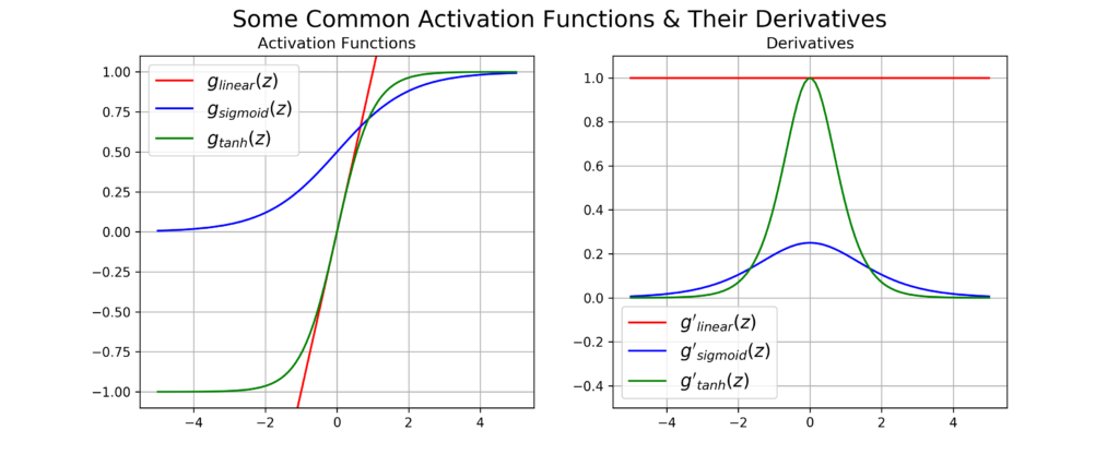
The vanishing/exploding gradient problem occurs because the inputs from preceding states are multiplied by the weights and pass through the activation function many times before reaching the final layer.

Source: https://dustinstansbury.github.io/theclevermachine/derivation-common-neural-network-activation-functions

If we take a look at the activation functions and their derivatives in the image above we can see that on the positive and negative limits the derivatives go to zero, except for the linear function (that no one uses, because it doesn’t introduce nonlinearity to the model). This way, you can imagine that an input being multiplied many times by a single value and being passed many times through an activation function would have small final derivative.

Because the update of the weights depend on the partial derivative of the input, if it is too small, the updates become too small too and this hurts the model’s performance. The exploding gradient has more to do with the way the weights are initialized, they could grow very large and the updates can become so large that the model never converges.

Some solutions can be applied to solve the problem presented:

  1. Use other activation functions, like ReLU. This activation function has a constant derivative, therefore, the gradient does not vanish (for a positive input);
  2. Gradient clipping: threshold the gradient to a value;
  3. Use Batch Normalization: this technique learns a normalization process to transform the output of each layer.

You can also try to change the model architecture to overcome this problem.

For the next article, I will be discussing the next architecture of Natural Language Models that came as an alternative to solve the problems imposed by the RNNs.

What is machine learning?

Machine learning is a branch of Artificial Intelligence and as such, it is a field that tries to create models to make better or faster decisions. Specifically, machine learning algorithms do that through analyzing data and adapting to it. As the model adapts, ideally it becomes more accurate in predicting.

Ok, but how is this useful?

The most useful cases of machine learning are cases where it is very difficult to formulate an algorithm to solve the problem. One example is the classification of objects in images. Imagine trying to create an algorithm to classify coffee beans as rotten or healthy, the color is important but also is how the beans can be oriented in the picture, at what distance they are from the camera (as that would affect their size in the image) and many other factors. This can turn out to be a near impossible task.

But how us humans can do it without even thinking? We have all these rules and patterns in our minds that were learned. And that is exactly what machine learning models will do. Essentially, every relevant aspect of the data (called feature), will be used by the model in a way that it tries to “understand” the effect of them in the expected result.

As you can imagine, the first thing to figure out is the question being asked. Is this a problem of prediction or classification? What am I interested in? Am I interested in knowing a number, for example, the temperature for tomorrow in my city or do I want to know if the coffee beans in an image are rotten or good for consumption?

Once framed the question, there must be a guarantee that the data at hand is reliable, it is clean and it’s sufficient for the needed accuracy of the model. As the complexity of the problem increases, so does the needed training sample size. Algorithms also are not intelligent as humans (yet) so they usually need a LOT of data to make sense of it and generalize well. A lot more than a human would need.

The learning methods

Machine learning algorithms have 4 types of learning methods: supervised, unsupervised, semi-supervised and reinforcement learning.

Supervised learning

The model uses labeled data to learn. What this means is that something (usually a human) has to tell the model what is what in the examples of the training/test sample. This learning method usually offers better accuracy than the unsupervised method but as it has the data requirement that it needs to be labeled, the data gathering process can be unfeasible. The targets of this type of models are either classes or numerical values. Use cases are very wide and the models can be theoretically used for anything that is divided in classes or is measured as a number.

Unsupervised learning

In this learning method, the model learns with unlabeled data, which means that it tries to identify similarities with the given data. Although this learning method produces less reliable results than supervised ones, they leverage the fact that unlabeled data that is much more easier to get. The targets of these models are associations (between data points) or clusters. Example of use cases are marketing customer profiles (clustering) for similar behaviour and related purchase items (association).

Semi-supervised learning

This method is a mix of the two, part of the data is labeled but the majority is not and can be useful if one has a lot of unlabeled data and sufficient labeled data to draw some conclusions about the unlabeled data. The labeled data is used to fit a model to predict the labels of the unlabeled data. Then, a supervised model can learn using the total data.

Reinforcement learning

Reinforcement learning uses a different approach for learning patterns: an agent takes different actions in an evironment and after evaluates if the result of those actions were good or bad, this way, it reinforces the good patterns and penalizes bad patterns. Situations where one can not determine if an action is good or bad are use cases for this method. The best and most common example is a game because the rules are clear, the target result is clear but the quality of the plays are not always clear. Other examples are walking (or flying) from point A to point B.

I hope you liked this post, feel free to comment and reach out!